According to [WayBack] Hightlight active row/column in Excel without using VBA? – Stack Overflow: no, but you do not need much code.
On my list of things to try is to combine both answers there into one.
–jeroen
Posted by jpluimers on 2020/04/02
According to [WayBack] Hightlight active row/column in Excel without using VBA? – Stack Overflow: no, but you do not need much code.
On my list of things to try is to combine both answers there into one.
–jeroen

Posted in Development, Excel, Office, Power User, Software Development | Leave a Comment »
Posted by jpluimers on 2020/03/31
As I need this one day:
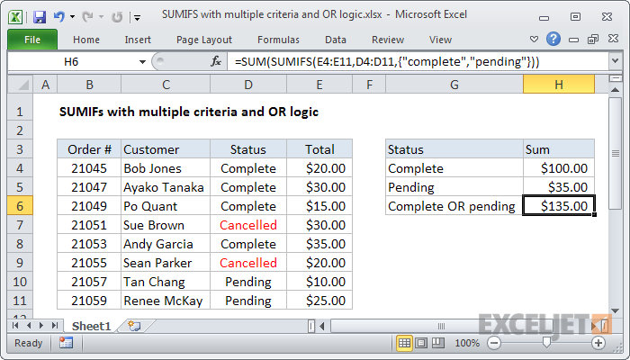
To sum based on multiple criteria using OR logic, you can use the SUMIFS function with an array constant. In the example shown, the formula in H6 is:
Source: [WayBack] Excel formula: SUMIFS with multiple criteria and OR logic | Exceljet
–jeroen

Posted in Development, Excel, Office, Office 2011 for Mac, Office 2013, Office 2016, Power User, Software Development | Leave a Comment »
Posted by jpluimers on 2020/03/18
The “Formulas” tab has to buttons that help to Display the relationships between formulas and cells – Excel [WayBack]:
- Precedent cells — cells that are referred to by a formula in another cell. For example, if cell D10 contains the formula =B5, then cell B5 is a precedent to cell D10.
- Dependent cells — these cells contain formulas that refer to other cells. For example, if cell D10 contains the formula =B5, cell D10 is a dependent of cell B5.
To assist you in checking your formulas, you can use the Trace Precedents and Trace Dependentscommands to graphically display and trace the relationships between these cells and formulas with tracer arrows, as shown in this figure.
Related:
–jeroen

Posted in Development, Excel, Office, Power User, Software Development | Leave a Comment »
Posted by jpluimers on 2020/03/13
[WayBack] worksheet function – How to add or subtract to, or increment, column letters in Excel? – Super User:
Here’s the best I’ve found so far:
=SUBSTITUTE(ADDRESS(1,( COLUMN() + 1 ),4),1,"")The part in the middle marked in bold is the only part that changes. In this example, it’s taking the current column and adding1, so returningBif it’s in columnAandAAif it’s in columnZ.
It is related to the question and answer [WayBack] Formula to return just the Column Letter in excel – Super User:
FYI on your original formula you don’t actually need to call the CELL formula to get row and column you can use:
=ADDRESS(ROW(),COLUMN())Then as an extension of that you can use MID & SEARCH to find the $ and trim down the output so you are just left with the letter:
=MID(ADDRESS(ROW(),COLUMN()),SEARCH("$",ADDRESS(ROW(),COLUMN()))+1,SEARCH("$",ADDRESS(ROW(),COLUMN()),SEARCH("$",ADDRESS(ROW(),COLUMN()))+1)-2)edit You can even simplify this further:
=MID(ADDRESS(ROW(),COLUMN()),2,SEARCH("$",ADDRESS(ROW(),COLUMN()),2)-2)
And it is part of a much more elaborate answer
Posted in Development, Excel, Office, Power User, Software Development | Leave a Comment »
Posted by jpluimers on 2019/11/22
 This indeed was an Excel 2011 for Mac thing.
Even without macros or VBA modules, Excel 2011 for Mac shows this dialog when opening a .xls file.
The solution was simple: save as .xlsx.
–jeroen
via [WayBack] Removing “Workbook Contains Macros” Prompt – Free Excel\VBA Help Forum

Posted in Excel, Office, Office 2011 for Mac, Power User | Leave a Comment »
Posted by jpluimers on 2019/11/19
I never thought you could do it, but you can: [Archive.is] Return empty cell from formula in Excel – Stack Overflow.
You have to crate:
Convoluted, but clever!
–jeroen
Posted in Development, Excel, Office, Office VBA, Power User, Software Development | Leave a Comment »
Posted by jpluimers on 2019/11/11
Lots of fuzz, but the formula towards the end worked:
=SUMPRODUCT(MID(0&A1,LARGE(INDEX(ISNUMBER(--MID(A1,ROW($1:$25),1))*

ROW($1:$25),0),ROW($1:$25))+1,1)*10^ROW($1:$25)/10)
Source: [Archive.is] How to Extract a Number or Text from Excel with this Function
More of those at [WayBack] Extract Only Numbers From Text String
–jeroen
Posted in Excel, Office, Office 2011 for Mac, Power User | Leave a Comment »
Posted by jpluimers on 2019/10/04
Sometimes in a table, you want to have a key column where one of the rows sorts after Z (for instance having a total value further on).
The A-Z sort order sorts all non-letter ASCII characters in front of A-Z and a-z because [WayBack] Excel sorting is not in ASCII order – Microsoft Community, see ASCII Sort.xlsm – Microsoft Excel Online.
Using =NA() (which displays as #N/A ) is too visually intrusive (but works, see: [WayBack] Forcing an item to sort last in Excel [Archive] – Actuarial Outpost)
Luckily, putting in an Arabic character like 'ٴ works. You can even put it in front of normaal ASCII characters like in 'ٴ ----- which then displays it at the right (since Arabic is Right-to-Left) -----ٴ .
The character is high Hamza – Wikipedia; [WayBack] Unicode Character ‘ARABIC LETTER HIGH HAMZA’ (U+0674)
via:
–jeroen
Posted in Excel, Office, Power User | Leave a Comment »
Posted by jpluimers on 2019/10/04
 Since I don’t do Excel visualisations often enough, I always forget the details on Pivot Charts, some links and tips below.
You can’t have enough axes
The tips below assume you can create a pivot table from an existing table (that already can contain formulas), then show you:
Creating graphs out of up and down time durations over time, aggregated by day.
Ideas for correlations that might matter:
First of all, I needed “day of month”, “day of week”, and “week number” so I could group by those. Based on Readable weekdays in Excel, you get formulas like these:
=DAY(B4)=WEEKDAY(B4) and =TEXT(B4;"dddd")=WEEKNUM(B4)Then I needed to split the duration of the state in distinct up/down durations. So I made a few formulas:
=("Up", A4) to have a boolean for up/down=("Up", A4) to have a boolean for up/down=IF(D4;C4;0)to split the up duration from the state duration=IF(NOT(D4);C4;0)to split the down duration from the state durationA pivot table could aggregate total up and down durations, but I wanted a measure of up ratio, so I needed a formula inside the pivot table itself.
Following the steps at [WayBack] Calculate values in a PivotTable Use different ways to calculate values in calculated fields in a PivotTable report in Excel 2010, I got to this one:
This aggregates nicely: drag it to the aggregates column, then change the aggregation to “Average”:

Posted in Excel, Office, Power User | Leave a Comment »
Posted by jpluimers on 2019/09/30
Since I always forget this: [WayBack] Exceljet: Get day name from date
If you need to get the day name (i.e. Monday, Tuesday, etc.) from a date, there are several options depending on your needs.
Basically there are four ways go get the day of the week; the first three are readable, but when ordered, they are ordered alphabetically. The last one is numeric.
Combining the numeric with the text is easier in for instance Pivot Legend Fields (Series).
So here they go (based on the above link), assuming that B4 contains a timestamp:
=WEEKDAY(B4) gives you the numeric weekday (starting with Sunday=1 to Saturday=7) which allows sorting in a meaningful order=TEXT(B4,"dddd") gives you the full day name of B4 in your locale=TEXT(B4,"ddd") gives you the shortened day name of B4 in your locale=CHOOSE(WEEKDAY(B4),"Sun","Mon","Tue","Wed","Thu","Fri","Sat") gives you a name of your liking from a series of 7 textsNote that depending on your locale, these formulas might actually need a semicolon:
=WEEKDAY(B4)=TEXT(B4;"dddd")=TEXT(B4;"ddd")=CHOOSE(WEEKDAY(B4);"Sun";"Mon";"Tue";"Wed";"Thu";"Fri";"Sat")–jeroen

Posted in Excel, Office, Power User | Leave a Comment »